Examples

These examples illustrate how to use the CBR-FoX library across different datasets and scenarios, showing the full workflow from loading data to visualization.

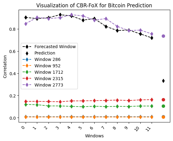
Bitcoin Prediction

1. Import Necessary Libraries

Import required modules and libraries

from cbr_fox.builder.cbr_fox_builder import cbr_fox_builder
from cbr_fox.core import cbr_fox
from cbr_fox.custom_distance.cci_distance import cci_distance
import numpy as np

2. Load the Saved Data

Load preprocessed Bitcoin prediction data from a npz file

data = np.load("../examples/Bitcoin_prediction/Bitcoin_Prediction.npz")

3. Retrieve Variables from the Data

Extract relevant variables for model training and prediction

training_windows = data['training_windows']
forecasted_window = data['forecasted_window']
target_training_windows = data['target_training_windows']
windowsLen = data['windowsLen'].item()  # Extract single value
componentsLen = data['componentsLen'].item()
windowLen = data['windowLen'].item()
prediction = data['prediction']

4. Define CBR-FoX Techniques

Set up the CBR-FoX techniques using a custom distance metric

techniques = [
    cbr_fox.cbr_fox(metric=cci_distance, kwargs={"punishedSumFactor": 0.5})
]

5. Build and Train the CBR-FoX Model

Initialize the model builder and train on the loaded data

p = cbr_fox_builder(techniques)
p.fit(training_windows = training_windows,
      target_training_windows = target_training_windows,
      forecasted_window = forecasted_window)

Sample output from the model training process

2025-08-27 12:56:19,487 - INFO - Analizando conjunto de datos
...
2025-08-27 12:56:21,055 - INFO - Análisis finalizado

6. Make Predictions

Generate predictions and obtain explanations for the forecasted data

p.predict(prediction = prediction, num_cases=3)

Sample terminal output showing prediction report

2025-08-27 12:56:23,598 - INFO - Generando reporte de análisis

7. Visualize Results

Visualize predictions using a line plot with scatter markers

p.visualize_pyplot(
    fmt = '--d',
    scatter_params={"s": 50},
    xtick_rotation=50,
    title="Bitcoin Prediction",
    xlabel="Time",
    ylabel="Value"
)

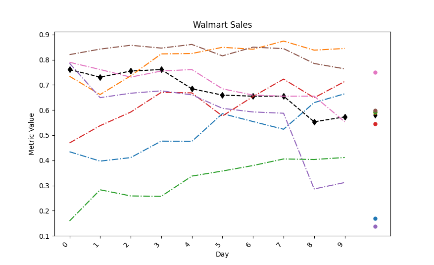
Walmart Sales Prediction

1. Load the Saved Data

Load Walmart sales data from a npz file

data = np.load("Walmart_Sales.npz")

2. Retrieve Variables from the Data

Extract variables required for training and forecasting

training_windows = data['training_windows']
forecasted_window = data['forecasted_window']
target_training_windows = data['target_training_windows']
windowsLen = data['windowsLen'].item()
componentsLen = data['componentsLen'].item()
windowLen = data['windowLen'].item()
prediction = data['prediction']

3. Define CBR-FoX Techniques

Set up CBR-FoX technique with CCI distance metric

techniques = [
    cbr_fox.cbr_fox(metric=cci_distance, kwargs={"punishedSumFactor": 0.5})
]

4. Build and Train the CBR-FoX Model

Initialize the model builder and train on Walmart data

p = cbr_fox_builder(techniques)
p.fit(training_windows = training_windows,
      target_training_windows = target_training_windows,
      forecasted_window = forecasted_window)

5. Make Predictions

Generate predictions for Walmart sales

p.predict(prediction = prediction, num_cases=3)

6. Visualize Results

Plot Walmart Sales predictions with customized markers

p.visualize_pyplot(
    fmt = '-.',
    legend = False,
    scatter_params={"s": 25},
    xtick_rotation=50,
    title="Walmart Sales",
    xlabel="Day",
    ylabel="Metric Value"
)

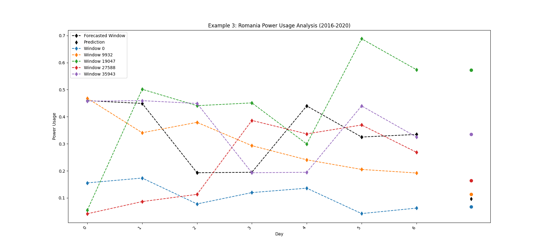
Romania Power Usage Prediction

1. Load the Saved Data

Load Romania Power Usage dataset from 2016-2020

data = np.load("Romania_Power_Usage_Analysis_2016_2020_CBR-FoX.npz")

2. Retrieve Variables from the Data

Extract training and prediction variables

training_windows = data['training_windows']
forecasted_window = data['forecasted_window']
target_training_windows = data['target_training_windows']
windowsLen = data['windowsLen'].item()
componentsLen = data['componentsLen'].item()
windowLen = data['windowLen'].item()
prediction = data['prediction']

3. Define CBR-FoX Techniques

Define multiple techniques with different punishedSumFactor values

techniques = [
    cbr_fox.cbr_fox(metric=cci_distance, kwargs={"punishedSumFactor":0.5}),
    cbr_fox.cbr_fox(metric=cci_distance, kwargs={"punishedSumFactor":0.7})
]

4. Build and Train the CBR-FoX Model

Train the model with multiple techniques on Romania dataset

p = cbr_fox_builder(techniques)
p.fit(training_windows = training_windows,
      target_training_windows = target_training_windows.reshape(-1,1),
      forecasted_window = forecasted_window)

5. Make Predictions

Generate predictions with 5 forecast cases

p.predict(prediction = prediction, num_cases=5)

6. Visualize Results

Visualize predictions with line plot and scatter markers

p.visualize_pyplot(
    fmt = '--d',
    scatter_params={"s": 50},
    xtick_rotation=50,
    title="Romania Power Usage",
    xlabel="Time",
    ylabel="Value"
)

Rainfall Prediction

1. Load the Saved Data

Load Rainfall prediction dataset from npz file

data = np.load("Rainfall_Prediction.npz")

2. Retrieve Variables from the Data

Extract variables for model training and forecasting

training_windows = data['training_windows']
forecasted_window = data['forecasted_window']
target_training_windows = data['target_training_windows']
windowsLen = data['windowsLen'].item()
componentsLen = data['componentsLen'].item()
windowLen = data['windowLen'].item()
prediction = data['prediction']

3. Define CBR-FoX Techniques

Set up CBR-FoX technique using CCI distance metric

techniques = [
    cbr_fox.cbr_fox(metric=cci_distance, kwargs={"punishedSumFactor": 0.5})
]

4. Build and Train the CBR-FoX Model

Initialize the builder and train the model on rainfall data

p = cbr_fox_builder(techniques)
p.fit(training_windows = training_windows,
      target_training_windows = target_training_windows,
      forecasted_window = forecasted_window)

5. Make Predictions

Generate rainfall predictions with 3 forecast cases

p.predict(prediction = prediction, num_cases=3)

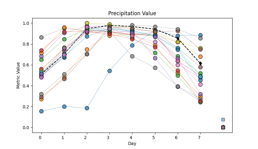
6. Visualize Results

Plot rainfall predictions with line and scatter markers

p.visualize_pyplot(
   fmt = '-o',
   plot_params = {"linewidth": .5,"alpha": 0.75,"markersize": 9,"markeredgecolor": "black"},
   legend = False,
   scatter_params = {"s": 45, "alpha": 0.5,"edgecolors": "black","marker":"s"},
   title="Precipitation Value",
   xlabel="Day",
   ylabel="Metric Value"
)

Weather Forecasting

1. Import Necessary Libraries

Import modules and dependencies for weather forecasting

from cbr_fox.core import cbr_fox
from cbr_fox.builder import cbr_fox_builder
from cbr_fox.custom_distance import cci_distance
import numpy as np
import os

2. Load the Saved Data

Load preprocessed weather forecasting dataset

data = np.load(os.path.join(os.path.dirname(__file__), "weather_forecasting.npz"))

3. Retrieve Variables from the Data

Extract input features and target variables

training_windows = data['training_windows']
forecasted_window = data['forecasted_window']
target_training_windows = data['target_training_windows']
windowsLen = data['windowsLen'].item()
componentsLen = data['componentsLen'].item()
windowLen = data['windowLen'].item()
prediction = data['prediction']

4. Define CBR-FoX Techniques

Define CBR-FoX technique with CCI distance

techniques = [
    cbr_fox.cbr_fox(metric=cci_distance, kwargs={"punishedSumFactor": 0.5})
    # cbr_fox.cbr_fox(metric="edr"),
    # cbr_fox.cbr_fox(metric="dtw"),
    # cbr_fox.cbr_fox(metric="twe")
]

5. Build and Train the CBR-FoX Model

Train model using weather forecasting dataset

p = cbr_fox_builder(techniques)
p.fit(training_windows = training_windows,
      target_training_windows = target_training_windows,
      forecasted_window = forecasted_window)

6. Make Predictions

Generate predictions for weather data

p.predict(prediction = prediction, num_cases=3)

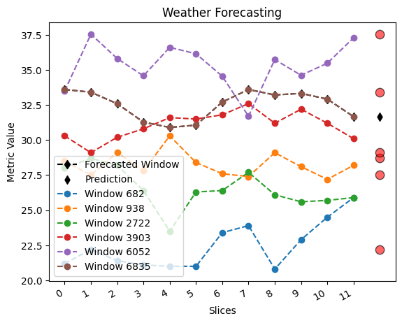
7. Visualize Results

Visualize weather forecast results with custom scatter plot

p.visualize_pyplot(
    fmt = '--o',
    legend = True,
    scatter_params = {"s": 80, "c": "red", "alpha": 0.6, "edgecolors": "black"},
    xtick_rotation = 30,
    title="Weather Forecasting",
    xlabel="Slices",
    ylabel="Metric Value"
)

Power consumption Forecasting

1. Import Necessary Libraries

Import modules and dependencies

from cbr_fox.core import cbr_fox
from cbr_fox.builder import cbr_fox_builder
from cbr_fox.custom_distance import cci_distance
import numpy as np
import os

2. Load the Saved Data

Load preprocessed Power Consumption dataset

data = np.load(os.path.join(os.path.dirname(__file__), "Power_consumption.npz"))

3. Retrieve Variables from the Data

Extract input features and target variables

training_windows = data['training_windows']
forecasted_window = data['forecasted_window']
target_training_windows = data['target_training_windows']
windowsLen = data['windowsLen'].item()
componentsLen = data['componentsLen'].item()
windowLen = data['windowLen'].item()
prediction = data['prediction']

4. Define CBR-FoX Techniques

Define CBR-FoX technique with CCI distance

techniques = [
    cbr_fox.cbr_fox(metric=cci_distance, kwargs={"punishedSumFactor": 0.5})
]

5. Build and Train the CBR-FoX Model

Train model using Power Consumption dataset

p = cbr_fox_builder(techniques)
p.fit(training_windows = training_windows,
      target_training_windows = target_training_windows,
      forecasted_window = forecasted_window)

6. Make Predictions

Generate predictions for Power consumption data

p.predict(prediction = prediction, num_cases=3)

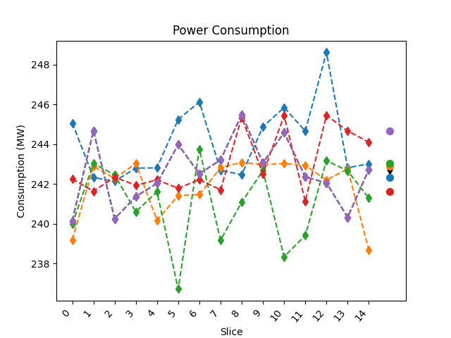
7. Visualize Results

Visualize weather forecast results with custom scatter plot

p.visualize_pyplot(
   fmt = '--d',
   legend = False,
   scatter_params={"s": 50},
   xtick_rotation=50,
   title="Power Consumption",
   xlabel="Slice",
   ylabel="Consumption (MW)"
)

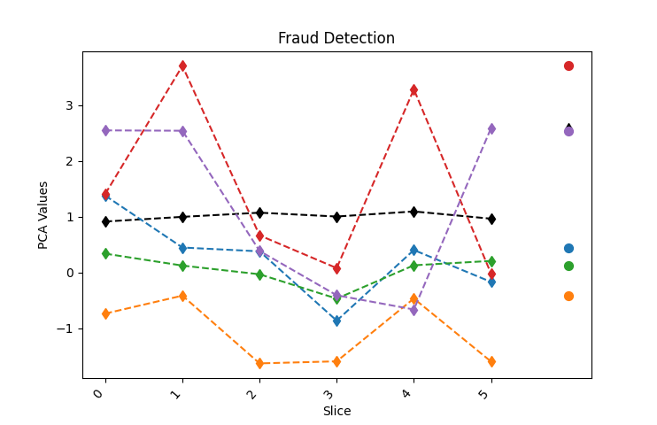
Fraud Detection

1. Import Necessary Libraries

Import modules and dependencies

from cbr_fox.core import cbr_fox
from cbr_fox.builder import cbr_fox_builder
from cbr_fox.custom_distance import cci_distance
import numpy as np
import os

2. Load the Saved Data

Load preprocessed Fraud Detection dataset

data = np.load(os.path.join(os.path.dirname(__file__), "Fraud_detection.npz"))

3. Retrieve Variables from the Data

Extract input features and target variables

training_windows = data['training_windows']
forecasted_window = data['forecasted_window']
target_training_windows = data['target_training_windows']
windowsLen = data['windowsLen'].item()
componentsLen = data['componentsLen'].item()
windowLen = data['windowLen'].item()
prediction = data['prediction']

4. Define CBR-FoX Techniques

Define CBR-FoX technique with CCI distance

techniques = [
    cbr_fox.cbr_fox(metric=cci_distance, kwargs={"punishedSumFactor": 0.6})
]

5. Build and Train the CBR-FoX Model

Train model using Fraud Detection dataset

p = cbr_fox_builder(techniques)
p.fit(training_windows = training_windows,
      target_training_windows = target_training_windows,
      forecasted_window = forecasted_window)

6. Make Predictions

Generate predictions for Fraud data

p.predict(prediction = prediction, num_cases=5)

7. Visualize Results

Visualize weather forecast results with custom scatter plot

p.visualize_pyplot(
   fmt = '--d',
   legend = False,
   scatter_params={"s": 50},
   xtick_rotation=50,
   title="Fraud Detection",
   xlabel="Slice",
   ylabel="PCA Values"
)